

The key pivot table shortcut keys in Excel are Ctrl+T to prepare the data, Alt, N, V, T to insert a PivotTable, Alt+F5 to refresh it and Alt+Shift+Right Arrow to group items. Add Alt+F1 for a PivotChart and you can build, update and chart a pivot table without leaving the keyboard.
Last updated: 14 November 2026. Compiled by Jitendra Rao, founder of Excel Keys, with 11+ years in MIS reporting and dashboard automation.
In this guide
- The 14 pivot table keys that save the most time
- A worked example with real numbers: 120 orders summarised by region
- Why a pivot table shows old numbers, and the key that fixes it
- How to group items and add a chart from the keyboard
- A free practice workbook with an answer key
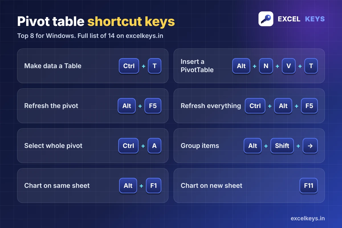
Pivot table shortcut keys at a glance
Click inside your data or PivotTable first. Most pivot keys only work when a cell inside the PivotTable is selected. Where a key has no Mac version, the Mac column says n/a.
| Windows | Mac | What it does |
|---|---|---|
Ctrl+T | Cmd+T | Turn the data into a Table, so the pivot picks up new rows |
Alt, N, V, T | n/a | Insert a PivotTable from a table or range (Excel 365) |
Alt, D, P | Cmd+Option+P | Open the classic PivotTable wizard |
Alt+F5 | n/a | Refresh the selected PivotTable |
Ctrl+Alt+F5 | n/a | Refresh all data in the workbook, including every PivotTable |
Ctrl+A | Cmd+A | Select the whole PivotTable |
Alt+↓ | Option+↓ | Open the filter list of the selected field |
Alt+Shift+→ | Cmd+Shift+K | Group the selected items |
Alt+Shift+← | Cmd+Shift+J | Ungroup the selected items |
Alt, J, T, L | n/a | Show or hide the PivotTable Field List |
Space | Space | Tick or untick the selected field in the Field List |
Alt+F1 | Option+F1 | Add a PivotChart on the same sheet |
F11 | F11 | Add a PivotChart on a new chart sheet |
Ctrl+Z | Cmd+Z | Undo the last change |
Worked example: 120 orders summarised by region
The free practice workbook has a Data sheet with 120 dummy sales orders: date, region, product, sales rep, units and amount. We want the total amount and the number of orders for each region.
- Make a Table. Click any cell in the data and press
Ctrl+T, then Enter. The data now has banded rows and filter buttons. - Insert the pivot. Press
Alt, thenN, thenV, thenT, one key at a time. Press Enter to put the PivotTable on a new sheet. - Choose the fields. Tick Region and Amount in the Field List. Region goes to Rows and Amount to Values.
- Read the result. The totals must match the Check sheet in the workbook, which uses SUMIFS formulas. They are in the table below.
| Region | Orders | Total amount |
|---|---|---|
| North | 37 | 2,446,500 |
| West | 27 | 1,653,100 |
| East | 25 | 1,582,500 |
| South | 31 | 912,500 |
| Grand total | 120 | 6,594,600 |
Add the four regions and you get 6,594,600, so the pivot is complete. One thing to notice: South places more orders than East (31 against 25) but earns less than 60% of East’s value. A pivot table makes a pattern like this visible in seconds, and it is the kind of question to take to the next sales review.
Why the pivot shows old numbers
A PivotTable is a snapshot. It does not update when the source data changes. Try it: in the Data sheet, change the Units for order ORD-1001 (South, Printer) from 4 to 5. A printer costs 9,500 in the dummy data, so the South total should rise by 9,500, from 912,500 to 922,000, and the grand total from 6,594,600 to 6,604,100. The pivot still shows the old numbers. Click inside it and press Alt+F5. Now the new totals appear.
If the workbook has several PivotTables or connections, press Ctrl+Alt+F5 to refresh them all. Microsoft’s help page on refreshing PivotTable data explains the other options, including refreshing when the file opens.
Group items from the keyboard
Remove the Region field, put Product in Rows, click Keyboard, hold Ctrl and click Monitor. Press Alt+Shift+Right Arrow. Excel creates a group called Group1 that holds both items, and you can rename it by typing over the name. Press Alt+Shift+Left Arrow to ungroup. This is useful for a report that needs “Accessories” instead of a long list of small products.
Add a chart in one key
Click a cell inside the pivot and press Alt+F1. A PivotChart appears on the same sheet. Press F11 instead to put it on its own chart sheet. Both charts follow the pivot: filter the pivot and the chart changes with it.
Common pivot table problems and fixes
- New rows are missing. The source range did not grow. Convert the data to a Table with Ctrl+T before you insert the pivot, then refresh with Alt+F5.
- The Field List disappeared. Click a cell inside the PivotTable and press Alt, J, T, L to bring it back.
- Group does nothing. The selected cells must be pivot items, not the values. Select the item names in the Rows area.
- Numbers are counted, not added. Excel counts a field if it has blank cells or numbers stored as text. Clean the column first. See our checklist on how to prepare Excel data for a dashboard.
A 5-day practice plan (10 minutes a day)
| Day | Keys to practise | Where |
|---|---|---|
| 1 | Ctrl+T, Alt, N, V, T | Data sheet, steps 1 and 2 |
| 2 | Space, Ctrl+A | Step 3, then select the whole pivot |
| 3 | Alt+F5, Ctrl+Alt+F5 | Step 4: change units and refresh |
| 4 | Alt+Shift+→, Alt+Shift+← | Step 5: group and ungroup products |
| 5 | Alt+F1, F11 | Step 6: charts, then compare with the Check sheet |
Download the free practice workbook (XLSX). It has an Instructions sheet, a Data sheet with 120 dummy orders and a Check sheet with live SUMIFS answers.
Once the pivot works, a dashboard is the next step. Our guide on how to create a dashboard in Excel shows how to connect charts to your pivot. For formula keys, read our Excel formula shortcut keys guide, and keep the A to Z shortcut list handy.
How this list was checked
- Ctrl+T, Ctrl+Alt+F5, Alt+F1 and F11 are on Microsoft Support’s Excel keyboard shortcuts, checked on 14 November 2026. Alt+F5 is covered in Microsoft’s help on refreshing PivotTable data.
- Alt, N, V, T, Alt+Shift+Arrow, Alt, J, T, L and the Space key come from standard pivot table shortcut references used by Excel trainers. Microsoft’s own page does not list them as a set.
- Every number in the worked example comes from the practice workbook, recalculated with no formula errors. Excel versions differ. If a key behaves differently on yours, email info@excelkeys.in with your Excel version.
Frequently asked questions
What is the shortcut to create a pivot table in Excel?
Select any cell in your data and press Alt, N, V, T one key after another. In Excel 365 this opens the PivotTable from table or range box. In some older versions Alt, N, V opens the dialog directly. The classic wizard opens with Alt, D, P.
What is the shortcut to refresh a pivot table?
Click any cell inside the PivotTable and press Alt+F5. To refresh every PivotTable and data connection in the workbook, press Ctrl+Alt+F5.
Why is my pivot table not updating when I change the data?
A PivotTable does not recalculate on its own. Press Alt+F5 after you change the source data. If you added new rows below the old range, the pivot may not include them. Turn the source data into a Table with Ctrl+T so the range grows automatically.
How do I select the whole pivot table with the keyboard?
Click any cell inside the PivotTable and press Ctrl+A. On a Mac, use Cmd+A. The selection covers the whole PivotTable, so you can copy it or clear it.
What is the shortcut to group items in a pivot table?
Select two or more text items and press Alt+Shift+Right Arrow to group them. Alt+Shift+Left Arrow ungroups them. You can also right-click and choose Group. On a Mac, use Cmd+Shift+K to group and Cmd+Shift+J to ungroup.
Do pivot table shortcut keys work on a Mac?
Some do: Cmd+T for a Table, Cmd+A to select the PivotTable, Option+F1 for a PivotChart, Cmd+Shift+K to group. Key-tip sequences such as Alt, N, V, T have no Mac version. On a Mac, use Insert > PivotTable from the ribbon.
Keep going
Open the full Excel shortcut keys list for 200+ keys, Windows and Mac side by side.
If your team needs a pivot-based report turned into a working dashboard, see the dashboards we have built.