Learning how to create a dashboard in Excel comes down to five steps: keep your data in one clean table, summarise it with SUMIFS and COUNTIFS, show the key numbers as KPI cards, add three or four charts, and arrange everything on one screen. This guide builds a working order dashboard you can download.
Key takeaways
- A dashboard is a one-screen summary: 3 to 5 KPI cards and 3 to 4 charts, nothing more.
- Keep raw data on its own sheet and let SUMIFS and COUNTIFS feed the dashboard, so it updates when you paste new rows.
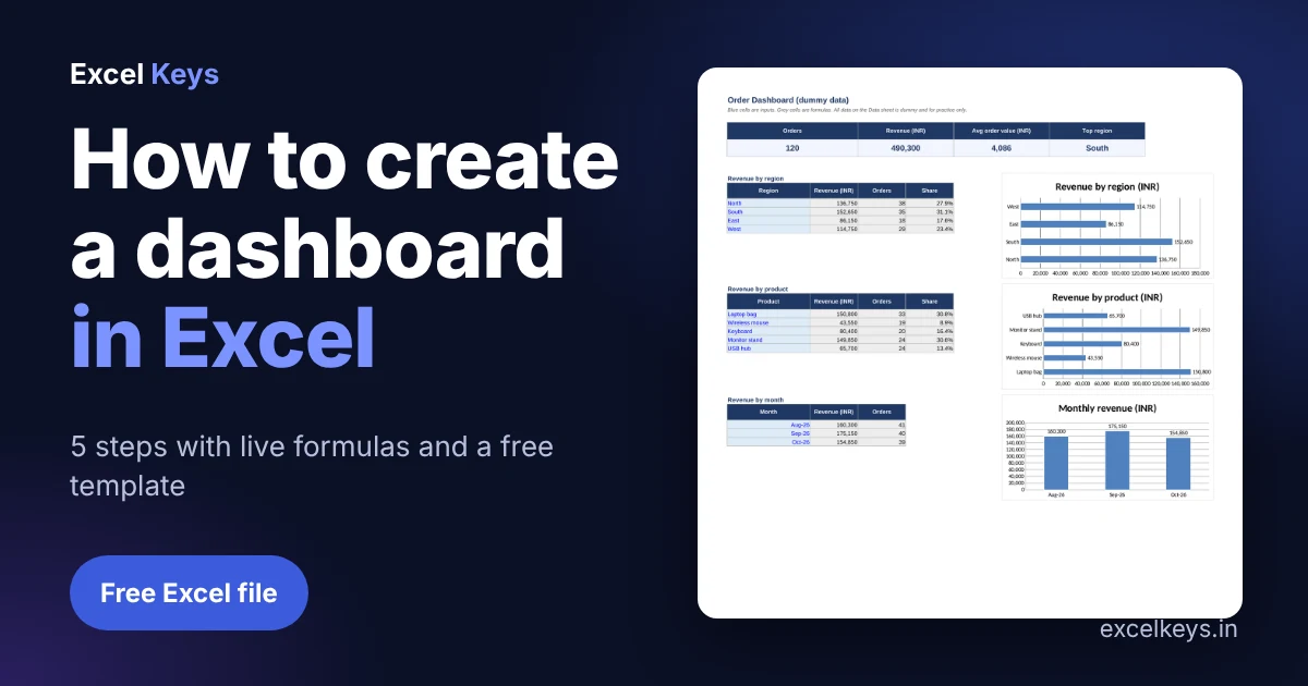
- In the free template, 120 dummy orders add up to Rs 490,300, an average order value of Rs 4,086.
- Prepare the data first. Most dashboard problems are data problems.
In this guide
- What makes a dashboard different from a report
- Step 1: Prepare the data
- Step 2: Build the summary tables with SUMIFS and COUNTIFS
- Step 3: Add KPI cards
- Step 4: Insert charts that answer one question each
- Step 5: Arrange the layout and share it
- Worked example: what the numbers say
- Download the free Excel dashboard template
- Common mistakes to avoid
- When to ask for a custom dashboard
- Frequently asked questions
What makes a dashboard different from a report
A report lists numbers. A dashboard answers a question at a glance: are we on track, which region is behind, which product carries the month. If you are new to the idea, read our guide to the MIS report in Excel first, because a dashboard is usually the visual layer on top of an MIS report.
Before you build anything, decide the one question the dashboard answers. For this example it is: where does our order revenue come from?
Step 1: Prepare the data
Put every order in one table with one header row, no merged cells, no blank rows and one value per cell. Dates must be real dates and amounts must be numbers. Our data preparation checklist covers this in detail, and it saves hours later.
| Order ID | Order date | Region | Product | Qty | Unit price | Amount |
|---|---|---|---|---|---|---|
| ORD-1001 | 01-Aug-26 | West | USB hub | 4 | 900 | 3,600 |
| ORD-1002 | 01-Aug-26 | West | USB hub | 2 | 900 | 1,800 |
Step 2: Build the summary tables with SUMIFS and COUNTIFS
Each chart needs a small summary table behind it. Type the categories (regions, products, months) in a column and calculate against the Data sheet. The workhorse is SUMIFS, which adds values that meet a condition. Order counts use COUNTIFS.
Revenue for the region in A10:
=SUMIFS(Data!$G$2:$G$500, Data!$C$2:$C$500, $A10)

Orders for the region in A10:
=COUNTIFS(Data!$C$2:$C$500, $A10)

Share of total:
=IFERROR(B10/SUM(B$10:B$13), 0)
Ranges run to row 500 so new rows are picked up without editing a formula. Monthly figures use a date range: the month start in column A and EDATE to find the next month.
=SUMIFS(Data!$G$2:$G$500, Data!$B$2:$B$500, ">="&$A34, Data!$B$2:$B$500, "<"&EDATE($A34,1))Step 3: Add KPI cards
KPI cards are single cells in a larger font that show the headline numbers. Four is plenty.
| KPI | Formula | Result (dummy data) |
|---|---|---|
| Orders | =COUNTA(Data!$A$2:$A$500) | 120 |
| Revenue | =SUM(Data!$G$2:$G$500) | Rs 490,300 |
| Average order value | =IFERROR(C5/A5,0) | Rs 4,086 |
| Top region | =INDEX(A10:A13,MATCH(MAX(B10:B13),B10:B13,0)) | South |
The IFERROR wrapper stops a divide-by-zero error from appearing when the sheet is empty. Details are in Microsoft’s guide to the IFERROR function.
Step 4: Insert charts that answer one question each
- Select a summary table, including its header.
- Insert a bar chart for categories with long names (products, regions) and a column or line chart for time.
- Delete the legend when there is one series, add data labels, and write a title that states the point, not just the topic.
- Use one colour. Reserve a second colour for the thing you want people to notice.
Microsoft lists every option in its page on available chart types. Skip 3-D and pie charts with more than four slices, because they make comparisons harder.
Step 5: Arrange the layout and share it
- KPI cards across the top, charts below, filters or notes at the side.
- Hide gridlines and the Data sheet if the audience only needs the dashboard.
- Check it at 100 percent zoom on a laptop screen. If you must scroll sideways, remove something.
- Highlight exceptions with rules. Our sister guide on conditional formatting in Excel shows how.
Worked example: what the numbers say
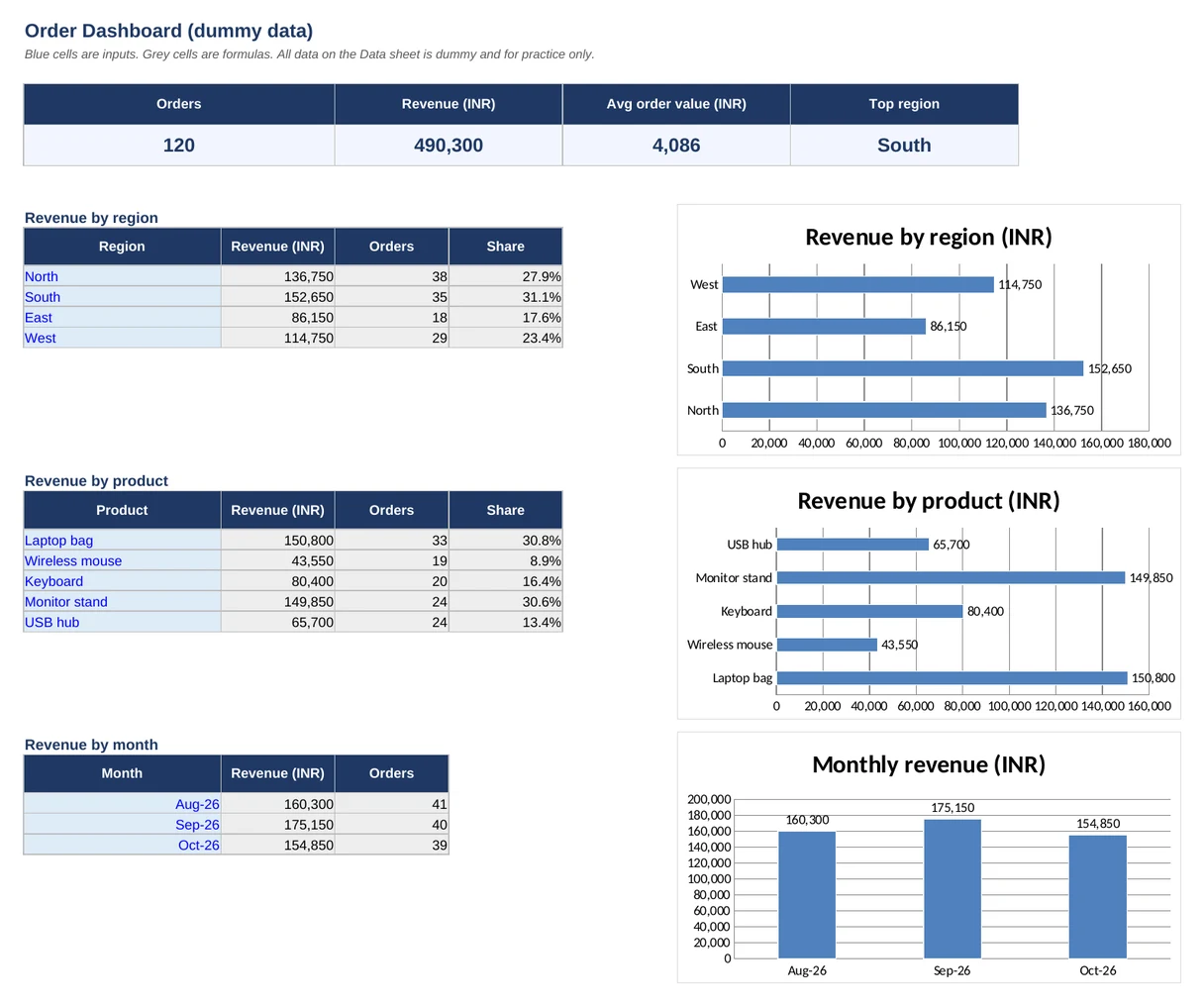
With 120 dummy orders from August to October 2026, total revenue is Rs 490,300 and the average order is Rs 4,086. By region, South leads with Rs 152,650 (31.1 percent), while East is lowest at Rs 86,150. By product, Laptop bag brings in Rs 150,800 and Wireless mouse brings Rs 43,550.
Monthly revenue runs Rs 160,300 in August, Rs 175,150 in September and Rs 154,850 in October. This is practice data, so use it to learn the method, then paste your own orders.
Download the free Excel dashboard template
Now that you know how to create a dashboard in Excel, the quickest way to learn is to open a finished one and change the data.
The file has the Data sheet, the Dashboard sheet with live formulas and charts, and a How to use sheet. There are no macros, so it opens safely in any recent Excel version.
Common mistakes to avoid
- Building charts straight on the raw data, so every new month means rebuilding.
- Typing totals by hand instead of using formulas.
- Merged cells and blank rows inside the data, which break SUMIFS and pivot tables.
- Putting ten charts on one screen. If everything is highlighted, nothing is.
- Choosing a tool before the question. Our comparison of Excel dashboards and Power BI helps you decide.
When to ask for a custom dashboard
Knowing how to create a dashboard in Excel covers most small teams. This template suits a single sheet of orders. When you have several source files, monthly refresh rules or many users, a built-to-order dashboard saves time. Excel Keys builds custom Excel dashboards that run offline on your own file, with no data leaving your computer. See the Business Performance Dashboard for an example, or contact us with your report.
Frequently asked questions
How do I create a dashboard in Excel from scratch?
Put your data in one clean table, build small summary tables with SUMIFS and COUNTIFS, show headline numbers as KPI cards, add three or four charts, and arrange them on one sheet. Keep the data on a separate sheet so the dashboard updates when new rows are pasted in.
Which Excel functions are best for dashboards?
SUMIFS, COUNTIFS, AVERAGEIFS, INDEX with MATCH, IFERROR and EDATE cover most dashboards. They work in every modern Excel version, so the file opens for colleagues who have older software, and they are easy to audit when a number looks wrong.
Do I need a pivot table or Power Query to make a dashboard?
No. Pivot tables are quick for exploring data, and Power Query helps when you combine files, but a formula-driven dashboard works well for one table of data. Start simple, and add Power Query only when cleaning or merging becomes a repeated chore.
How many charts should a dashboard have?
Three to four charts and three to five KPI cards is a good limit. Each chart should answer one clear question. If a viewer has to scroll or study the screen to find the message, remove the least useful chart.
Is the free dashboard template safe to open?
Yes. The file has no macros and uses only dummy data. It contains standard formulas and charts, so it opens in Excel 2016 or later. Replace the dummy rows with your own orders, and keep your own copy for each month.
About the author: Jitendra Rao is the founder of Excel Keys and has spent over 11 years building MIS reports, sales analytics and dashboard automation for banking and finance teams. He builds Excel dashboards that run offline, on your own files. Last updated: 11 November 2026.