
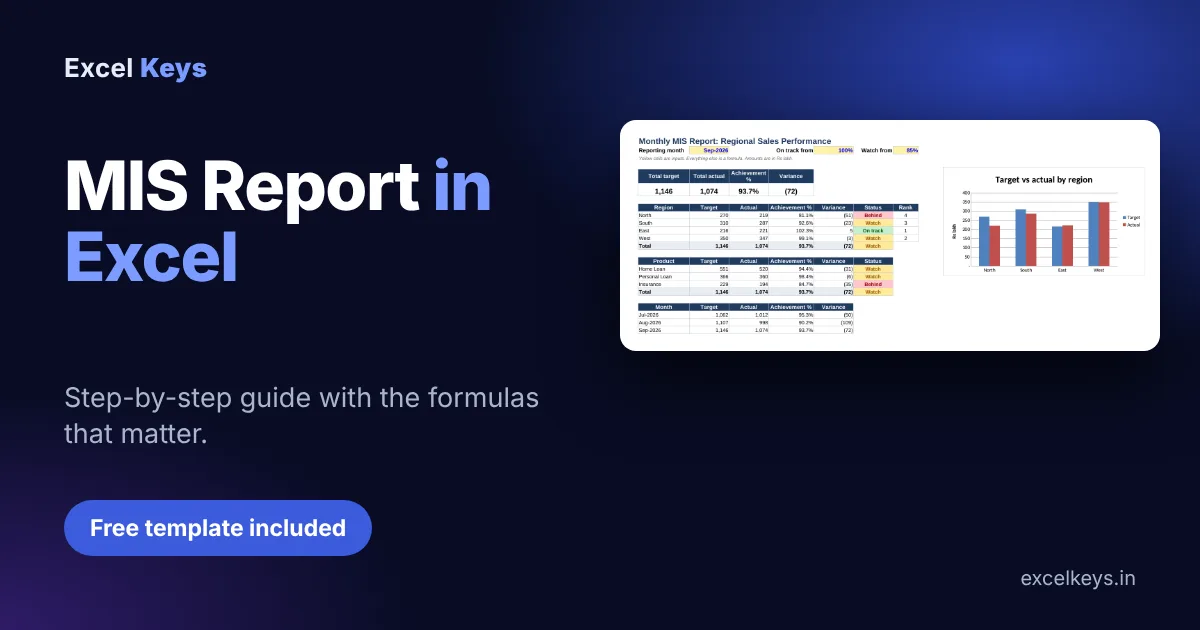
An MIS report in Excel is the one-page monthly summary your manager actually reads: what the target was, what really happened, and where the gap sits. Most teams build it by hand every month and lose half a day to copy-paste. This guide shows how to build it once, with five formulas, so that changing a single cell refreshes the whole report.
You can follow along with the finished workbook. Jump to the free MIS report template if you would rather start from a working file.
Key takeaways
- An MIS report answers three questions: what was planned, what happened, and where the gap is.
- Keep raw data on one sheet and the report on another, so the report never has to be retyped.
- Five formulas cover most of it: SUMIFS, achievement %, variance, an IF status flag and RANK.
- One input cell for the reporting month lets the same report show any month you choose.
- Use a PivotTable to explore data, and formulas for the fixed monthly layout your manager expects.
In this guide
- What is an MIS report in Excel?
- What a good MIS report contains
- How to make an MIS report in Excel, step by step
- Worked example: reading the numbers
- Free MIS report template
- PivotTable or formulas?
- Common mistakes
- Frequently asked questions
What is an MIS report in Excel?
An MIS (management information system) report in Excel is a structured summary that turns raw business records, such as sales, collections or hiring data, into a few numbers a manager can act on: target, actual, achievement percentage, variance and trend. It usually has one data sheet and one summary sheet that updates when a new month is added.
MIS stands for management information system, the combination of data, tools and routines an organisation uses to support decisions (Wikipedia has a short overview). In day-to-day work, though, “MIS report” simply means the periodic summary that goes to a sales head, branch manager, HR head or operations lead. Banks, insurers, NBFCs and distribution teams in India produce them daily, weekly and monthly.
In my 11+ years of building MIS reports for sales and banking teams, the weak point is almost never the formulas. It is the layout: raw data and report mixed on one sheet, totals typed by hand, and a new file created each month.
What a good MIS report contains
A useful MIS report is short. Each block on the page should answer one question, and each block should be one formula pattern you can copy.
| Section | Question it answers | Excel tool |
|---|---|---|
| Headline KPIs | How are we doing overall this month? | SUMIFS, SUM |
| Breakdown by region, product or team | Where is the gap coming from? | SUMIFS with one more condition |
| Achievement % | How close are we to target? | Actual ÷ Target |
| Variance | By how many rupees are we ahead or behind? | Actual − Target |
| Status flag | Which items need attention first? | IF + conditional formatting |
| Rank | Who is leading and who is trailing? | RANK |
| Trend | Is it getting better or worse? | EDATE + SUMIFS |
| One chart | Can the manager see it in five seconds? | Clustered bar chart |
Keep it to one printable page. If your manager has to scroll to find the answer, you have built a data dump, not an MIS report.
How to make an MIS report in Excel, step by step
The steps below use the free template, which holds dummy sales figures in Rs lakh for four regions and three products across three months. Replace them with your own export and the report follows.
Step 1: Put the raw data on its own sheet
Create a sheet named Data with one header row and one row per record. The template uses five columns: Month, Region, Product, Target and Actual. Store the month as a real date (the first day of the month), keep amounts as numbers, and never add total rows. If your data arrives messy, the checklist for preparing Excel data takes ten minutes and saves hours later.
If you want the report to grow automatically as you add rows, convert the data to an Excel Table. The template uses fixed ranges to row 37 and tells you where to extend them.
Step 2: Add one input cell for the reporting month
On the MIS Summary sheet, reserve a single cell (B2 in the template) for the reporting month and type the first day of the month, for example 01-Sep-2026. Every formula below refers to this cell. To produce last month’s report you change one date, not twenty formulas.
Step 3: Pull target and actual with SUMIFS
SUMIFS adds numbers that meet one or more conditions. For the headline cards, the only condition is the month:
Total target:  =SUMIFS(Data!$D$2:$D$37, Data!$A$2:$A$37, $B$2)
Total actual:  =SUMIFS(Data!$E$2:$E$37, Data!$A$2:$A$37, $B$2)
For the region table, add a second condition so each row picks up its own region from column A:
Target for North:  =SUMIFS(Data!$D$2:$D$37, Data!$B$2:$B$37, $A9, Data!$A$2:$A$37, $B$2)
Actual for North:  =SUMIFS(Data!$E$2:$E$37, Data!$B$2:$B$37, $A9, Data!$A$2:$A$37, $B$2)
The dollar signs lock the ranges, so you can copy the formula down to every region. For the product table, point the condition at the Product column (column C of the Data sheet) instead of Region.
Step 4: Calculate achievement % and variance
Achievement %:  =IF(B9=0, 0, C9/B9)
Variance:       =C9-B9
Always guard the division. A region with no target this month would otherwise show a #DIV/0! error in the middle of a report you are about to send. Format achievement as a percentage and variance with brackets for negatives, so a shortfall such as (51) stands out.
Step 5: Add a status flag with IF
Managers scan colours before they read numbers. Put the two thresholds in input cells (E2 and G2 in the template) rather than inside the formula, so you can change them without editing every row:
=IF(D9>=$E$2, "On track", IF(D9>=$G$2, "Watch", "Behind"))With thresholds of 100% and 85%, a region at 92.6% shows “Watch” and one at 81.1% shows “Behind”. Then add conditional formatting (green, amber, red fills) to the Status column.
Step 6: Rank the regions
=RANK(D9, $D$9:$D$12)RANK returns 1 for the highest achievement and counts downwards. It is a small touch, but it answers “who is leading?” without anyone sorting the table.
Step 7: Show a three-month trend
A single month hides direction. Use EDATE to step back from the reporting month, then reuse SUMIFS:
Month 1 (two months back):  =EDATE($B$2, -2)
Month 2 (last month):       =EDATE($B$2, -1)
Month 3 (reporting month):  =EDATE($B$2, 0)
Target for that month:      =SUMIFS(Data!$D$2:$D$37, Data!$A$2:$A$37, $A22)
Step 8: Add one chart and set up the print page
Select the region names with their Target and Actual columns and insert a clustered bar chart. Then set the sheet to landscape and “fit to one page wide” so the report prints or exports to PDF exactly as it appears on screen.
Worked example: reading the numbers
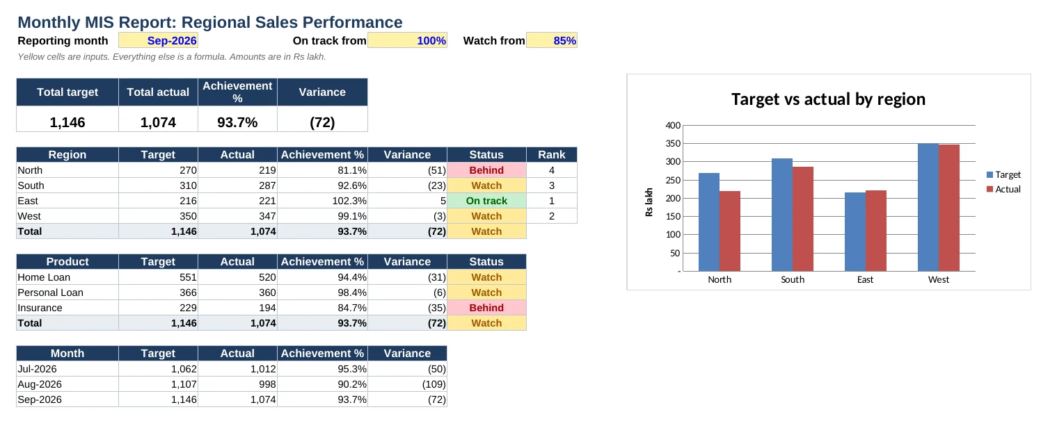
Here is the September 2026 report from the template. All values are dummy figures in Rs lakh, created only to demonstrate the layout.
| Region | Target | Actual | Achievement % | Variance | Status | Rank |
|---|---|---|---|---|---|---|
| North | 270 | 219 | 81.1% | (51) | Behind | 4 |
| South | 310 | 287 | 92.6% | (23) | Watch | 3 |
| East | 216 | 221 | 102.3% | 5 | On track | 1 |
| West | 350 | 347 | 99.1% | (3) | Watch | 2 |
| Total | 1,146 | 1,074 | 93.7% | (72) | Watch |
Read it the way a manager would. The company is at 93.7% of target, which looks like a mild miss. But North alone is 51 lakh short, and the total shortfall is 72 lakh, so one region explains about 71% of the gap. West is only 3 lakh short, which is a rounding error next to North.
That is the real job of an MIS report: not to show numbers, but to point at the one place where a conversation is needed. The three-month trend in the same sheet adds context. Total achievement was 95.3% in July, 90.2% in August and 93.7% in September, so September is a recovery, not a slide.
Free MIS report template (download)
The workbook used in this guide is free to download and adapt for your own reporting. It has three sheets: Data (dummy records you replace with your export), MIS Summary (all formulas, status colours and the chart) and How to use (instructions and assumptions).
- Yellow cells are inputs; everything else is a formula.
- Change the reporting month in B2 and the whole report, including the trend, updates.
- Edit the status thresholds in E2 and G2 to match your own targets.
- Add regions or products in column A of the summary and the formulas pick them up.
The template uses only classic functions (SUMIFS, IF, RANK, EDATE), so it works in every modern version of Excel without add-ins or macros.
PivotTable or formulas: which should you use for MIS?
Both work, and good analysts use both. A PivotTable is the fastest way to explore data. Formulas are better when the report layout is fixed and the same page goes to the same people every month.
| Question | PivotTable | Formula-based report |
|---|---|---|
| Best for | Exploring and slicing data quickly | A fixed layout sent every month |
| Refresh | Needs a manual Refresh after new data | Updates as soon as the data or the month cell changes |
| Layout control | Limited (pivot style) | Full control, including status flags and thresholds |
| Learning curve | Low to start, harder to customise | Moderate: SUMIFS and IF are enough |
| Risk | Stale numbers if you forget to refresh | Broken ranges if the data grows past the formula range |
My rule of thumb: explore in a PivotTable, then publish from formulas.
Common mistakes to avoid in an MIS report
- Mixing data and report on one sheet. Every new month then means deleting and re-pasting, and eventually something breaks.
- Typing totals by hand. A hard-coded total is wrong the moment one row changes. Use SUM or SUMIFS.
- Dates stored as text. SUMIFS will match nothing and return zero. Check that the month column is a real date.
- Inconsistent names. “North” and “North ” (with a trailing space) are two regions to Excel. Use drop-downs for entry.
- Unguarded division. Wrap achievement formulas in IF(target=0, 0, …) so one empty row does not show an error.
- Too many numbers. If everything is highlighted, nothing is. Show the few KPIs that drive decisions.
- No assumptions noted. Write the unit (Rs lakh, Rs crore) and the definition of achievement on the sheet itself.
When to go beyond a template
A template is enough for one team and a few thousand rows. When data arrives from several systems, when the report must be emailed to many managers, or when you need drill-downs by branch and relationship manager, a purpose-built dashboard is faster and safer. See how we handle this in our RM productivity dashboard and business performance dashboard projects, and read the comparison of a custom Excel dashboard and Power BI before you decide on a tool.
If you would like an MIS report built around your own data and targets, send us a message with a sample of your file (dummy values are fine) and we will tell you what it would take.
Frequently asked questions
How do I create an MIS report in Excel?
Put your raw records on a Data sheet, add a summary sheet with a reporting-month cell, then use SUMIFS to pull target and actual, formulas for achievement % and variance, an IF for status, and a chart. Changing the month cell refreshes the whole report.
What should an MIS report include?
At minimum: target, actual, achievement percentage, variance, a status flag and a short trend, broken down by the dimension your manager is responsible for, such as region, product or team. Keep it to one printable page and add one clear chart.
Which Excel formulas are most useful for MIS reports?
SUMIFS and COUNTIFS for totals by condition, IF for status flags, RANK for leaderboards, EDATE for month-on-month trends and INDEX with MATCH for lookups. These classic functions work in every modern version of Excel without any add-ins.
Is a PivotTable better than formulas for an MIS report?
Neither is always better. A PivotTable is fastest for exploring data, while formulas suit a fixed monthly layout with status flags and thresholds. Many analysts explore in a PivotTable first and then publish the final report from formulas.
How do I automate a monthly MIS report in Excel?
Keep data on one sheet, drive the report from a single month cell and use formulas instead of pasted values. Each month you paste the new export and change the date. When data comes from several files, Power Query or a dashboard saves more time.
Can I download a free MIS report template in Excel?
Yes. The Excel Keys template on this page is free to download. It includes a data sheet, a formula-driven summary with status colours and a chart, and a how-to sheet. Replace the dummy data with your own figures and the report updates.
Build your MIS report once, reuse it every month
A good MIS report in Excel is not about clever formulas. It is about a clean data sheet, one input cell and a summary that points at the problem. Download the template, replace the dummy rows with your own and you will have a working monthly report in under an hour.
About the author: Jitendra Rao is the founder of Excel Keys and has spent over 11 years building MIS reports, sales analytics and dashboard automation for banking and finance teams. He builds Excel dashboards that run offline, on your own files. Last updated: 13 October 2026.